Introducing hs-speedscope - a way to visualise time profiles
Posted on November 7, 2019
In GHC-8.10 it will become possible to use speedscope to visualise the performance of a Haskell program. speedscope is an interactive flamegraph visualiser, we can use it to visualise the output of the -p profiling option. Here’s how to use it:
- Run your program with
prog +RTS -p -l-au. This will create an eventlog with cost centre stack sample events. - Convert the eventlog into the speedscope JSON format using
hs-speedscope. Thehs-speedscopeexecutable takes an eventlog file as the input and produces the speedscope JSON file. - Load the resulting
prog.eventlog.jsonfile into speedscope.app.
Using Speedscope
Speedscope then has three modes for viewing the profile. The default mode shows you the executation trace of your program. The call stack extends downwards, the wider the box, the more time was spent in that part of the program. You can select part of the profile by selecting part of the minimap, zoom using +/- or pan using the arrow keys. The follow examples are from profiling GHC building Cabal:
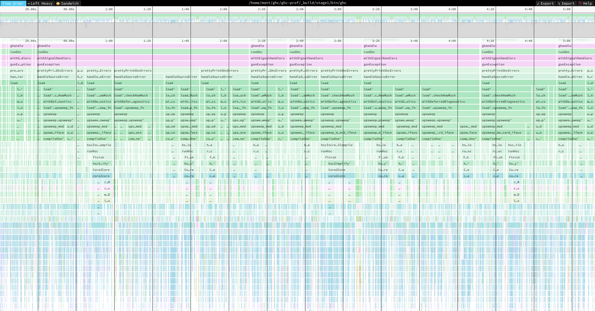
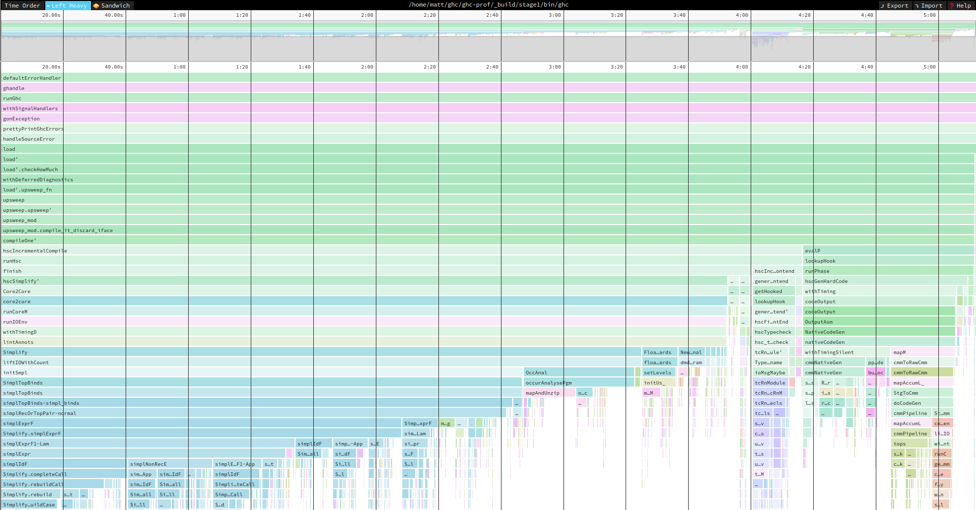
The first summarised view is accessed by the “left-heavy” tab. This is like the summarised output of the -p flag. The cost centre stacks which account for the most time will be grouped together at the left of the view. This way you can easily see which executation paths take the longest over the course of the whole executation of the program.
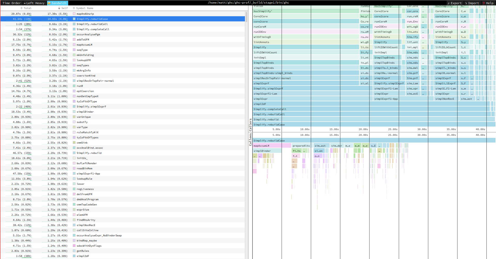
Finally, the “sandwich” view tries to work out which specific cost centre is responsible for the most executation time. You can use this to try to understand the functions which take the most time to execute. How useful this view is depends on the resolution of your cost centres in your program. Speedscope attempts to work out the most expensive cost centre by subtracting the total time spent beneath that cost centre from the time spent in the cost centre. For example, if f calls g and h, the cost of in f is calculated by the total time for f minus the time spend in g and h. If the cost of f is high, then there is some computation happening in f which is not captured by any further cost centres.
How is this different to the other profile visualisers?
The most important difference is that I didn’t implement the visualiser, it is a generic visualiser which can support many different languages. I don’t have to maintain the visualiser or work out how to make it scale to very big profiles. You can easily load 60mb profiles using speedscope without any rendering problems. All the library does is directly convert the eventlog into the generic speedscope JSON format.
How is this different to the support already in speedscope?
If you consult the documentation for speedscope you will see that it claims to support Haskell programs already. Rudimentary support has already been implemented by using the JSON output produced by the -pj flag but the default view which shows an executation trace of your program hasn’t worked correctly because the output of -pj is too generalised. If you program ends up calling the same code path many different times during the executation of the program, they are all identified in the final profile.
The second important difference is that each capability will be displayed on a separate profile. This makes profiling more useful for parallel programs.
How does it work?
I added support to dump the raw output from -p to the eventlog. Now it’s possible to process the raw information in order to produce the format that speedscope requires.